The Rosenblatt Perceptron: Zero to Hero
This is the first post in a series where we read foundational ML papers and make them intuitive. The goal: by the end, you should understand what the paper was really about—not just the math, but the ideas.
Paper: Frank Rosenblatt, “The Perceptron: A Probabilistic Model for Information Storage and Organization in the Brain” (1958)
The Problem: Drawing a Line
Forget neural networks for a moment. Here’s a simpler question.
You have a bunch of points on a 2D plane. Some are blue, some are red. Can you draw a straight line that separates them?
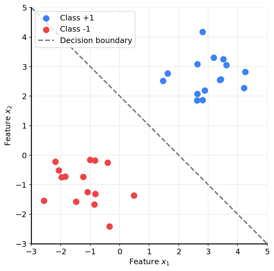
This is called linear classification. The line is a decision boundary—everything on one side is “blue,” everything on the other side is “red.”
If someone gives you a new point, you just check which side of the line it falls on. Done.
But here’s the hard part: how do you find the right line?
You could eyeball it. But what if there are thousands of points? What if it’s not 2D but 100-dimensional? What if you need a machine to do it automatically?
That’s what the perceptron solves.
The Perceptron: A Weighted Vote
The perceptron is the simplest possible classifier. It works like this:
- Take the input (e.g., coordinates of a point)
- Multiply each input by a weight
- Add them up (plus a bias term)
- If the sum is positive, output +1. Otherwise, output -1.
That’s it. Mathematically:
\[\hat{y} = \text{sign}(w_1 x_1 + w_2 x_2 + b)\]Where:
- $x_1, x_2$ are the input features
- $w_1, w_2$ are the weights (learnable)
- $b$ is the bias (also learnable)
- $\text{sign}$ returns +1 if the sum is ≥ 0, else -1
Here’s what it looks like as a diagram:

An Analogy: The Judge
Think of it like a judge scoring evidence in a trial.
Each piece of evidence has a weight (how important is it?). The judge adds up all the weighted evidence. If the total exceeds a threshold, the verdict is “guilty.” Otherwise, “not guilty.”
The perceptron is this judge. The weights encode what matters. The bias is the threshold.
The question is: who decides the weights?
Learning: Turning the Knobs
Here’s where it gets interesting. The perceptron doesn’t need you to specify the weights. It learns them from examples.
Imagine an old radio with analog dials. You don’t know the exact frequency of the station you want—you just twist the knobs until the static clears and you hear music.
The perceptron works the same way:
- Start with random weights (or zeros)
- Feed in a training example
- If the prediction is wrong, nudge the weights in the right direction
- Repeat until the line separates the classes
The key insight: you don’t need to know the right answer in advance. You just need feedback on whether you’re wrong, and a rule for how to correct yourself.
The Update Rule: Step by Step
The learning rule is simple:
If the prediction is wrong, update the weights:
\(w \leftarrow w + \eta \cdot y \cdot x\) \(b \leftarrow b + \eta \cdot y\)
Where:
- $y$ is the true label (+1 or -1)
- $\hat{y}$ is the prediction
- $\eta$ is the learning rate (a small number like 0.1)
- $x$ is the input
If $y = \hat{y}$ (correct), do nothing.
Why This Works (Intuition)
If a positive example ($y = +1$) was misclassified as negative, we add the input to the weights. This increases $w \cdot x$ for similar inputs, making them more likely to be classified as positive.
If a negative example ($y = -1$) was misclassified as positive, we subtract the input from the weights. This decreases $w \cdot x$ for similar inputs.
Each update pushes the decision boundary in the right direction.
Worked Example: Training Step by Step
Let’s trace through it with actual numbers. We’ll use learning rate $\eta = 0.1$.
Initial state: $w = [0, 0]$, $b = 0$

Let’s walk through the key steps:
Step 1: Input $[2, 1]$, label $+1$
- Compute: $0 \cdot 2 + 0 \cdot 1 + 0 = 0$
- Prediction: $\text{sign}(0) = +1$ (we’ll say sign(0) = +1)
- Correct! No update needed.
Step 2: Input $[-1, -1]$, label $-1$
- Compute: $0 \cdot (-1) + 0 \cdot (-1) + 0 = 0$
- Prediction: $\text{sign}(0) = +1$
- Wrong! True label is $-1$.
- Update: $w \leftarrow [0, 0] + 0.1 \cdot (-1) \cdot [-1, -1] = [0.1, 0.1]$
- Update: $b \leftarrow 0 + 0.1 \cdot (-1) = -0.1$
Now $w = [0.1, 0.1]$, $b = -0.1$.
Step 3: Input $[1, 2]$, label $+1$
- Compute: $0.1 \cdot 1 + 0.1 \cdot 2 - 0.1 = 0.2$
- Prediction: $\text{sign}(0.2) = +1$
- Correct! No update.
And so on. After enough passes through the data, the weights converge to values that correctly separate the classes.
The Geometric View: A Moving Line
Here’s the beautiful part. The weights $w = [w_1, w_2]$ define a line:
\[w_1 x_1 + w_2 x_2 + b = 0\]Every time we update the weights, the line moves.
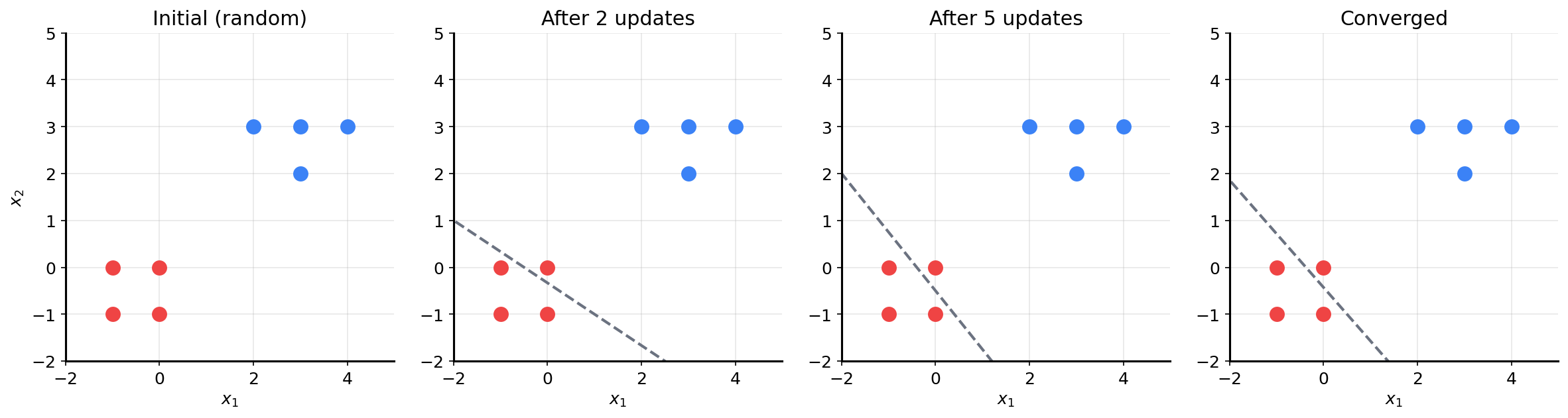
The line rotates and shifts with each mistake until it finds a position that separates all the points.
Going back to the radio analogy: each misclassification is feedback that you’re not tuned in yet. You keep adjusting until the signal is clear.
The Convergence Theorem
Here’s the remarkable part: if the data is linearly separable, the perceptron will find a separating line. Guaranteed.
This is Rosenblatt’s convergence theorem. The proof isn’t important for intuition, but the implication is:
- The knob-turning process doesn’t wander forever
- It converges in a finite number of steps
- The perceptron will always find a solution (if one exists)
This was a big deal in 1958. A machine that learns from examples and is guaranteed to succeed? That felt like magic.
Python Implementation
Let’s implement it. About 25 lines of clean code.
import numpy as np

class Perceptron:
    def __init__(self, lr=0.1, epochs=20):
        self.lr = lr
        self.epochs = epochs
        self.w = None
        self.b = 0.0

    def predict(self, x):
        return 1 if np.dot(self.w, x) + self.b >= 0 else -1

    def fit(self, X, y):
        n_features = X.shape[1]
        self.w = np.zeros(n_features)
        self.b = 0.0

        for _ in range(self.epochs):
            for xi, yi in zip(X, y):
                y_hat = self.predict(xi)
                if yi != y_hat:
                    self.w += self.lr * yi * xi
                    self.b += self.lr * yi
Training on Our Example
X = np.array([
    [2, 1], [3, 3], [4, 2],    # Class +1
    [-1, -1], [-2, -1], [-1, 0] # Class -1
])
y = np.array([1, 1, 1, -1, -1, -1])

model = Perceptron(lr=0.1, epochs=10)
model.fit(X, y)

for xi, yi in zip(X, y):
    print(f"{xi} -> predicted: {model.predict(xi)}, actual: {yi}")
You should see all predictions matching the true labels.
Where It Breaks: The XOR Problem
Now the catch.
Consider these four points:
| $x_1$ | $x_2$ | Label |
|---|---|---|
| 1 | 1 | +1 |
| 1 | -1 | -1 |
| -1 | 1 | -1 |
| -1 | -1 | +1 |
This is the XOR function. Can you draw a single line that separates the +1 points from the -1 points?
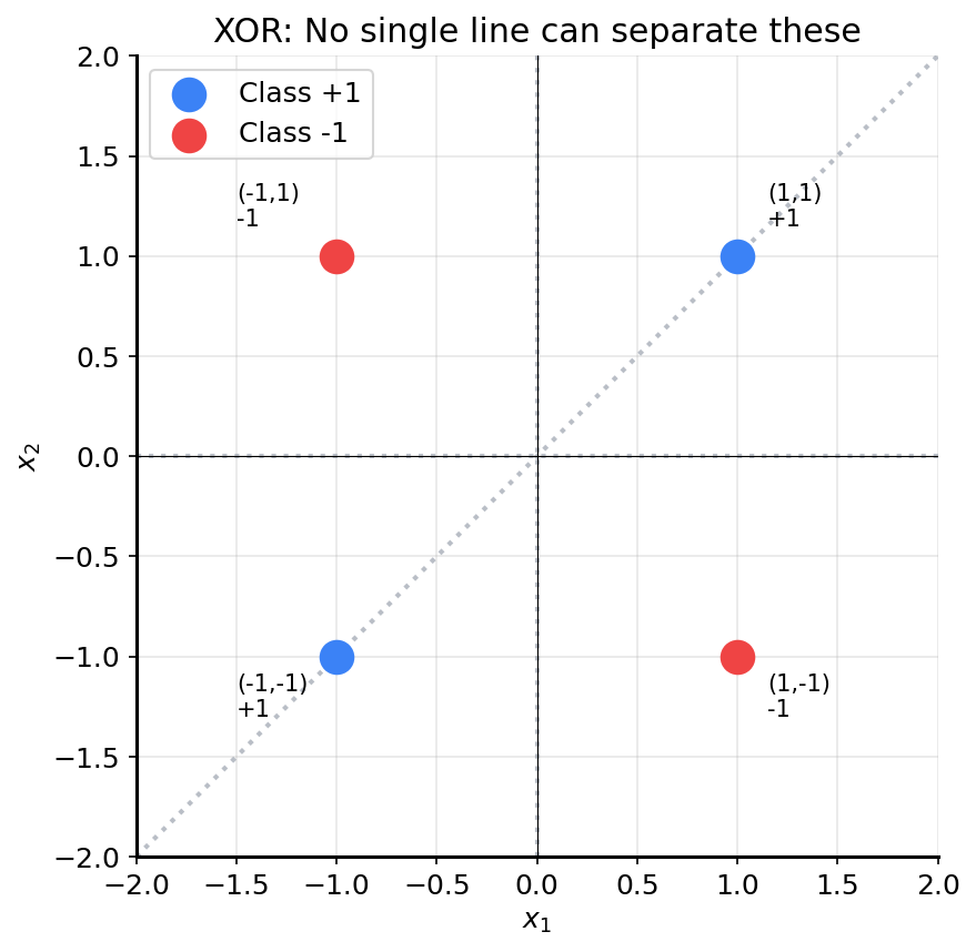
No matter how you tilt or shift the line, you can’t separate them. The classes are interleaved.
The perceptron can only learn linearly separable patterns. XOR is not linearly separable.
This isn’t a bug—it’s a fundamental limitation. And understanding this limitation is what eventually led to multi-layer networks (the “deep” in deep learning).
What Rosenblatt Actually Proposed
Now that you understand the perceptron, let’s connect back to the paper.
Rosenblatt wasn’t just building a classifier. He was modeling how brains might learn.
His full model had three layers:
- S-units (Sensory): Raw input, like pixels on a retina
- A-units (Association): Combine raw inputs into features. A single A-unit might respond to “an edge in this region” or “brightness above threshold”
- R-units (Response): The final decision—what class does this input belong to?
The key insight: the wiring between S and A units is random. Rosenblatt didn’t hand-engineer features. He let the randomness create a diverse set of feature detectors, then learned which combinations mattered for classification.
This is why the paper was revolutionary:
- No explicit programming of rules
- Learning from experience
- Emergent recognition from simple components
The Paper’s Lasting Ideas
Even though the single-layer perceptron has limitations, Rosenblatt’s framing introduced ideas that persist today:
Memory as probability, not templates. The perceptron doesn’t store a perfect copy of each training example. It adjusts weights—changing the probability that similar inputs will be classified the same way.
Generalization through shared structure. Similar inputs activate overlapping pathways. If I’ve learned that “edges in this region” predict cats, I can recognize new cat images with similar edge patterns.
The perceptron is the atom. Everything else—multi-layer perceptrons, CNNs, transformers—is built from this same primitive: weighted sum + activation. If you understand why the perceptron works and why it fails, you understand the foundation of neural networks.
Next Up
The perceptron can’t solve XOR. So what do we do?
We stack perceptrons. A second layer can compute features that the first layer can’t see. This lets us draw curved (or more complex) boundaries.
But now we have a new problem: how do we update the weights in the hidden layer? There’s no direct error signal—only the output layer sees the true label.
That’s the problem backpropagation solves. And that’s what we’ll cover next.
If you want more diagrams, a deeper dive into convergence proofs, or other variations (voted perceptron, kernel perceptron), let me know and I’ll add them.